
Surrogate-Based Optimization
Surrogate-based optimization represents a class of optimization methodologies that make use of surrogate modeling techniques to quickly find the local or global optima. It provides us a novel optimization framework in which the conventional optimization algorithms, e.g. gradient-based or evolutionary algorithms are used for sub-optimization.
For optimization problems, surrogate models can be regarded as approximation models for the cost function and state function, which are built from sampled data obtained by randomly probing the design space. Once the surrogate models are built, an optimization algorithm can be used to search the new candidate, based on the surrogate models, that is most likely to be the optimum. Since the prediction with a surrogate model is generally much more efficient than that with a numerical analysis code, the computational cost associated with the search based on the surrogate models is generally negligible. Surrogate modeling is referred to as a technique that makes use of the sampled data to build surrogate models, which are sufficient to predict the output of an expensive function at untried points in the feasibility space. Thus, how to choose sample points, how to build surrogate models, and how to evaluate the accuracy of surrogate models are key issues for surrogate optimization.
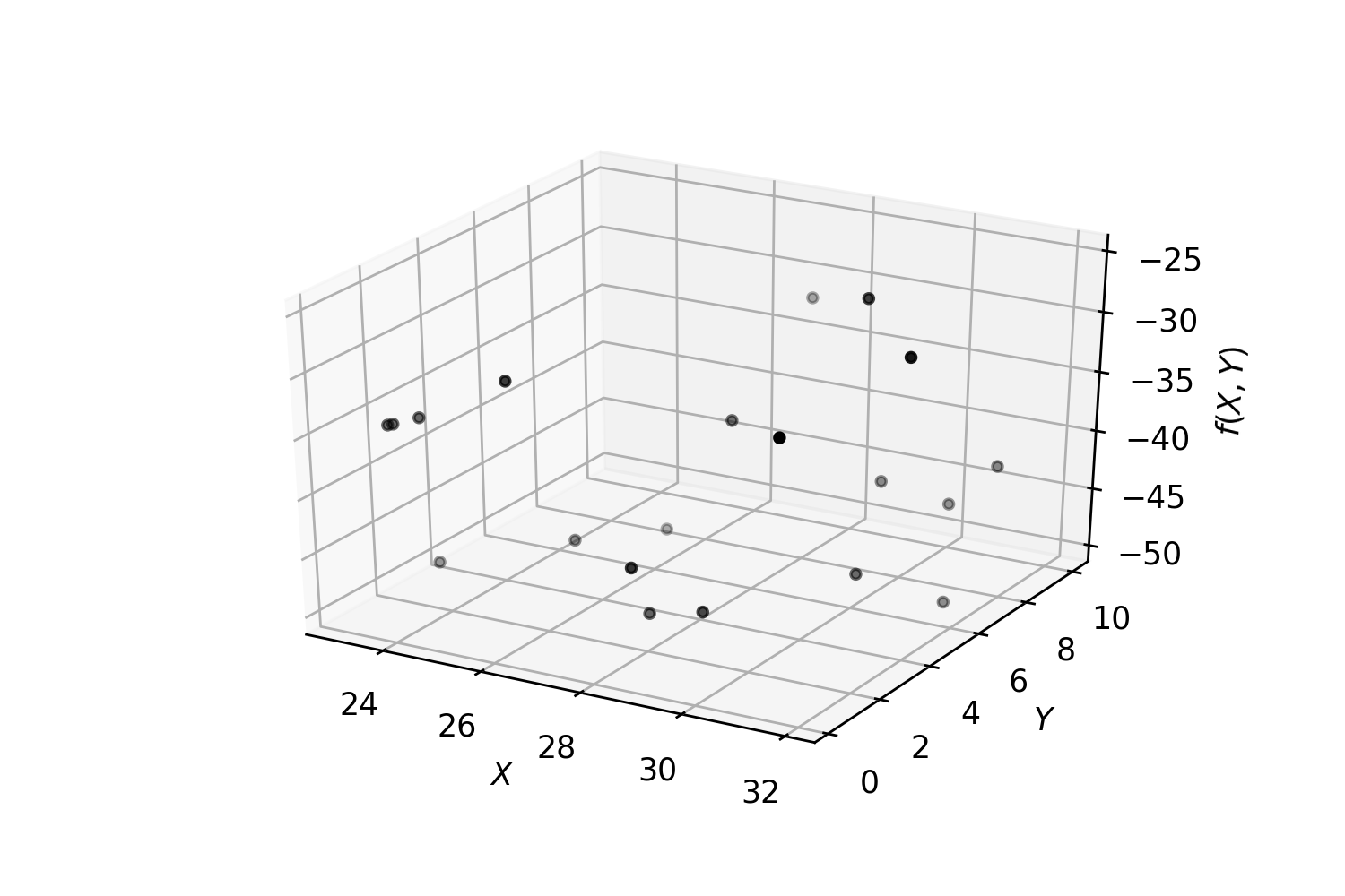
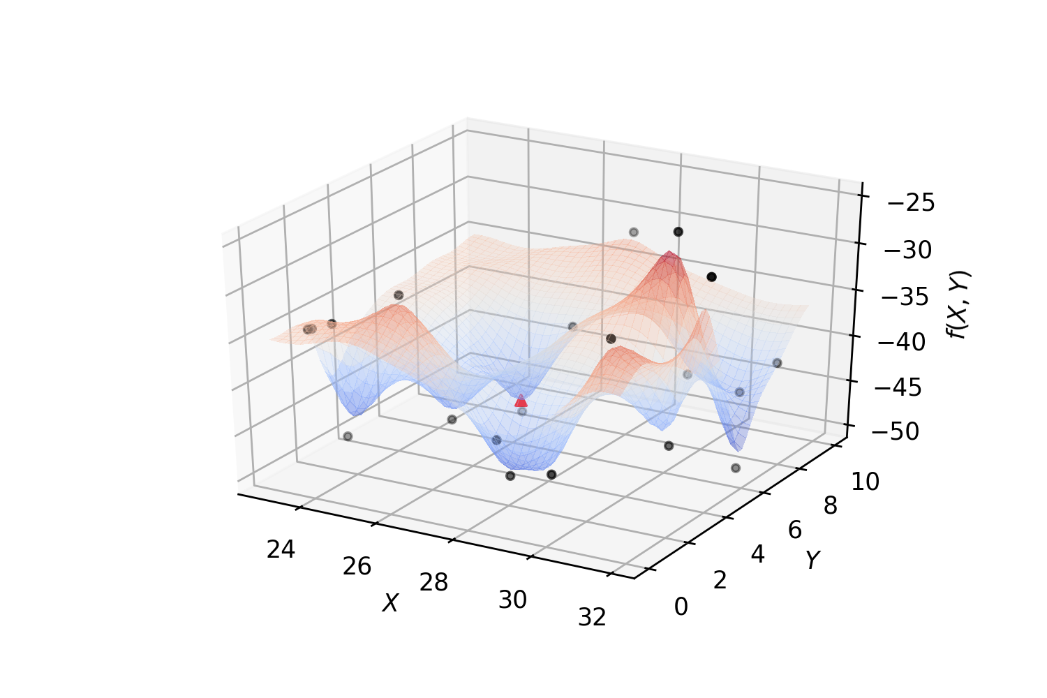
Fit a regressor and find a (local) minimum:
The following algorithm summarizes implemented Surrogate-Based Optimization for an expensive function \(f\) that can only be evaluated MaxIter times with a minimum MinEvals random evaluations.
Note
set \(E=\emptyset\), \(NumIter=0\)
while \(NumIter<MaxIter\) do
sample a random point \(x_0\) from feasible space
- if \(\#(E) < MinEvals\) then
- update \(E=E\cup\{(x_0, f(x_0))\}\)
- else
find a surrogate \(\hat{f}\) that fits the points in \(E\)
find the minimum \(x_*\) of \(\hat{f}\) using \(x_0\) as the initial point (if required)
evaluate \(f\) at \(x_*\) and update \(E=E\cup\{(x_*, f(x_*))\}\)
update \(NumIter = NumIter+1\)
return the pair \((x, y)\in E\) with lowest found value for \(y\) as the approximation for the minimum of \(f\)
Clearly, there are various methods to accomplish some of the steps in the above algorithm like how to sample a new point \(x_0\), how to find the surrogate \(\hat{f}\), how to minimize and how to decide when we wish to use the surrogate.
Sampling
Three different sampling methods have been implemented and the SurrogateSearch class accepts user defined sampling classes that have a certain signature.
CompactSample
This class samples a random point from the feasibility set.
BoxSample
This class samples a random point from a cube centered around a given point (usually the last point \(f\) was evaluated on) with a given length. It makes sure that the sample belongs to the feasibility set.
The length of the edges of the cube can be provided by setting init_radius (default: 2.)
A contraction ratio can be provided by setting contraction (should be bigger than 0 and less than 1) to shrink the volume of the cube to assure fast convergence to a (local) optima (default value: 0.9).
SphereSample
This class samples a random point from a sphere centered around a given point (usually the last point \(f\) was evaluated on) with a given radius. It makes sure that the sample belongs to the feasibility set.
The radius of the sphere can be provided by setting init_radius (default: 2.)
A contraction ratio can be provided by setting contraction (should be bigger than 0 and less than 1) to shrink the radius of the sphere to assure fast convergence to a (local) optima (default value: 0.9).
Note
The sampling method can be passed to an instance of SurrogateSearch via sampling parameter. Along with sampling class, radius, contraction, ineq, and bounds may be provided to be used by the sampling class. ineq is a list of callables which represent the constraints. bounds is a list of tuples of real numbers representing the bounds on each variable.
Tip
A user-defined sampling class should follow the following structure:
class UserSample(object):
    def __init__(self, **kwargs):
        pass

    def check_constraints(self, point):
        """
        Checks constraints on the sample if provided;
        `point` is the candidate to be checked;
        should return a `boolean` True or False for if all constraints hold or not.
        """
        pass

    def sample(self, centre, cntrctn=1.):
        """
        Samples a point out of an sphere centered at `centre`;

        `centre` is a `numpy.array` the center of the sphere;
        `cntrctn` is a  `float` customized contraction factor
        returns a `numpy.array` the new sample
        """
        pass
Surrogate models
By default, SurrogateSearch uses a polynomial surface of degree 3 to approximate \(f\) based on existing data and will be updated on each iteration where a new piece of information a bout \(f\) is found. Typically, any regressor inherited from RegressorMixin that implements a fit and a predict method can be used.
Optimizer
A scipy optimizer can be used to find a minimum of the surrogate at each iteration. Note that if ineqs is not None, then most of scipy optimizers can not be used. The optimizers that work well with constraints include ‘SLSQP’ and ‘COBYLA’.
An alternative for the scipy optimizer is ‘Optimithon’.
Hyperparameter Optimization
Hyperparameter Optimization in machine learning with respect to a given performance measure (e.g., accuracy, f1, auc, …) usually is a computationally expensive task which fits within the scope of surrogate optimization technique. In fact this is the main reason that the project exists. Therefore, there is a special class designed for hyperparameter optimization of machine learning methods that follow the schema of the very popular machine learning library scikit-learn. The class structsearch.SurrogateRandomCV is a substitute for scikit-learn’s GridSearchCV or RandomizedSearchCV. An isntance of SurrogateRandomCV takes an estimator like GridSearchCV and RandomizedSearchCV and a params parameter, like param_grid or param_distributions, which determines (ranges of) the values each argument of the estimator can take over. The difference is that not only it accepts discrete list of values for each parameter, it also accepts ranges of integers and real numbers too. The params is a dictionary whose keys are the estimator’s arguments and their values are objects of the followin types:
- Real(a, b): an interval of real numbers between \(a\) and \(b\);
- Integer(a, b): an interval of integer numbers between \(a\) and \(b\);
- Categorical(list): a list consists of discrete values;
- HDReal(a, b): An n dimensional box of real numbers corresponding to the classification groups (e.g. class_weight). a is the tuple of lower bounds and b is the tuple of upper bounds.
Example The following code searches for the best values for a SVC:
from sklearn.svm import SVC
from SKSurrogate import *
clf = SVC()
params = {'C': Real(1.e-5, 10),
          'kernel': Categorical(['poly', 'rbf']),
          'degree': Integer(1, 4),
          'gamma': Real(1.e-5, 10),
          'class_weight': HDReal((1.e-3, 1.e-3), (10., 10.))}
srch = SurrogateRandomCV(clf, params)
srch.fit(X, y)
print(srch.best_estimator_)
Note
It is worth mentioning that using a Gaussian Process Regression as the regressor simulates a particular variation of the optimization method known as Bayesian Optimization method.
Bayesian Optimization is the method employed by the popular package
skopt. The ui implemented for SurrogateRandomCV
is very much similar to the one of skopt.BayesSearchCV, so one could use the same code
for both given that the imports are carefully done.
Tip
The class SurrogateRandomCV works with intervals to handel the hyperparameters and
the current sampling classes do not impose extra constraints on SurrogateSearch other
than ranges for parameters, alternative scipy.minimize solvers can be used as well, such
as L-BFGS-B, TNC, SLSQP.