Hilbert Spaces
Orthonormal system of functions
Let X be a topological space and \(\mu\) be a finite Borel measure on X. The bilinear function \(\langle\cdot,\cdot\rangle\) defined on \(L_2(X, \mu)\) as \(\langle f, g\rangle = \int_X fg d\mu\) is an inner product which turns \(L_2(X, \mu)\) into a Hilbert space.
Let us denote the family of all continuous real valued functions on a non-empty compact space X by \(\textrm{C}(X)\). Suppose that among elements of \(\textrm{C}(X)\), a subfamily A of functions are of particular interest. Suppose that A is a subalgebra of \(\textrm{C}(X)\) containing constants. We say that an element \(f\in\textrm{C}(X)\) can be approximated by elements of A, if for every \(\epsilon>0\), there exists \(p\in A\) such that \(|f(x)-p(x)|<\epsilon\) for every \(x\in X\). The following classical results guarantees when every \(f\in\textrm{C}(X)\) can be approximated by elements of A.
Let \((V, \langle\cdot,\cdot\rangle)\) be an inner product space with \(\|v\|_2=\langle v,v\rangle^{\frac{1}{2}}\). A basis \(\{v_{\alpha}\}_{\alpha\in I}\) is called an orthonormal basis for V if \(\langle v_{\alpha},v_{\beta}\rangle=\delta_{\alpha\beta}\), where \(\delta_{\alpha\beta}=1\) if and only if \(\alpha=\beta\) and is equal to 0 otherwise. Every given set of linearly independent vectors can be turned into a set of orthonormal vectors that spans the same sub vector space as the original. The following well-known result gives an algorithm for producing such orthonormal from a set of linearly independent vectors:
Note
Gram–Schmidt
Let \((V,\langle\cdot,\cdot\rangle)\) be an inner product space. Suppose \(\{v_{i}\}^{n}_{i=1}\) is a set of linearly independent vectors in V. Let
and (inductively) let
Then \(\{u_{i}\}_{i=1}^{n}\) is an orthonormal collection, and for each k,
Note that in the above note, we can even assume that \(n=\infty\).
Let \(B=\{v_1, v_2, \dots\}\) be an ordered basis for \((V,\langle\cdot,\cdot\rangle)\). For any given vector \(w\in V\) and any initial segment of B, say \(B_n=\{v_1,\dots,v_n\}\), there exists a unique \(v\in\textrm{span}(B_n)\) such that \(\|w-v\|_2\) is the minimum:
Note
Let \(w\in V\) and B a finite orthonormal set of vectors (not necessarily a basis). Then for \(v=\sum_{u\in B}\langle u,w\rangle u\)
Now, let \(\mu\) be a finite measure on X and for \(f,g\in\textrm{C}(X)\) define \(\langle f,g\rangle=\int_Xf g d\mu\). This defines an inner product on the space of functions. The norm induced by the inner product is denoted by \(\|\cdot\|_{2}\). It is evident that
which implies that any good approximation in \(\|\cdot\|_{\infty}\) gives a good \(\|\cdot\|_{2}\)-approximation. But generally, our interest is the other way around. Employing Gram-Schmidt procedure, we can find \(\|\cdot\|_{2}\) within any desired accuracy, but this does not guarantee a good \(\|\cdot\|_{\infty}\)-approximation. The situation is favorable in finite dimensional case. Take \(B=\{p_1,\dots,p_n\}\subset\textrm{C}(X)\) and \(f\in\textrm{C}(X)\), then there exists \(K_f>0\) such that for every \(g\in\textrm{span}(B\cup\{f\})\),
Since X is assumed to be compact, \(\textrm{C}(X)\) is separable, i.e., \(\textrm{C}(X)\) admits a countable dimensional dense subvector space (e.g. polynomials for when X is a closed, bounded interval). Thus for every \(f\in\textrm{C}(X)\) and every \(\epsilon>0\) one can find a big enough finite B, such that the above inequality holds. In other words, good enough \(\|\cdot\|_{2}\)-approximations of f give good \(\|\cdot\|_{\infty}\)-approximations, as desired.
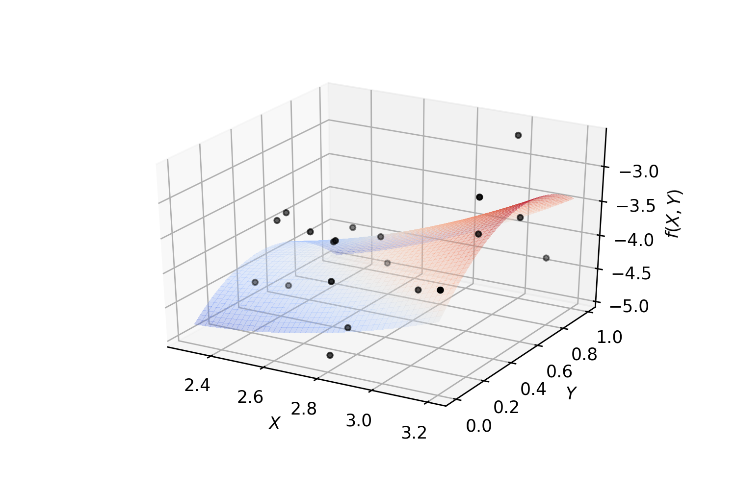
Example. Polynomial regression on 2-dimensional random data:
from mpl_toolkits.mplot3d import Axes3D
from matplotlib import cm
import matplotlib.pyplot as plt
import numpy as np
from SKSurrogate.NpyProximation import HilbertRegressor, FunctionBasis
def randrange(n, vmin, vmax):
        '''
        Helper function to make an array of random numbers having shape (n, )
        with each number distributed Uniform(vmin, vmax).
        '''
        return (vmax - vmin)*np.random.rand(n) + vmin

# degree of polynomials
deg = 2
FB = FunctionBasis()
B = FB.Poly(2, deg)
# initiate regressor
regressor = HilbertRegressor(base=B)
# number of random points
n = 20
fig = plt.figure()
ax = fig.add_subplot(111, projection='3d')
for c, m, zlow, zhigh in [('k', 'o', -5, -2.5)]:
        xs = randrange(n, 2.3, 3.2)
        ys = randrange(n, 0, 1.0)
        zs = randrange(n, zlow, zhigh)
        ax.scatter(xs, ys, zs, c=c, s=10, marker=m)
ax.set_xlabel('$X$')
ax.set_ylabel('$Y$')
ax.set_zlabel('$f(X,Y)$')
X = np.array([np.array((xs[_], ys[_])) for _ in range(n)])
y = np.array([np.array((zs[_],)) for _ in range(n)])
X_ = np.arange(2.3, 3.2, 0.02)
Y_ = np.arange(0, 1.0, 0.02)
_X, _Y = np.meshgrid(X_, Y_)
# fit the regressor
regressor.fit(X, y)
# prepare the plot
Z = []
for idx in range(_X.shape[0]):
        _X_ = _X[idx]
        _Y_ = _Y[idx]
        _Z_ = []
        for jdx in range(_X.shape[1]):
                t = np.array([np.array([_X_[jdx], _Y_[jdx]])])
                _Z_.append(regressor.predict(t)[0])
        Z.append(np.array(_Z_))
Z = np.array(Z)
surf = ax.plot_surface(_X, _Y, Z, cmap=cm.coolwarm, linewidth=0, antialiased=False, alpha=.3)