A machine learning progress tracker

When exploring for reasonable methods to model a problem, usually the search quickly results in a large number of candidates and it becomes very difficult to keep track of all models and their performance measures. There are various existing solutions, usually forcing to follow a particular workflow, which could be very beneficial. The present module tends to be very light, with minimal dependency and minimal effect of the workflow.

mltrace loves the scikit-learn compatible models and provides many tools to work with them. The vision and hence design of mltrace is based on the believe that most machine learning projects can be turned into a study on a certain dataset. Although, as the project progresses, features may be added to or dropped from the original data, but in most cases there is a systematic method to derive these changes from the original source. Therefore, mltrace isolates a task together with a dataset and the associated models.

Let us make up a sample classification task and trace the models via mltrace.

Step 0. Make a sample classification dataset:

# import requires libraries
import numpy as np
import pandas as pd
from sklearn.datasets import make_classification
from SKSurrogate import *
# make up a classification dataset
X, y = make_classification(n_samples=1000, n_features=10, n_informative=6, n_redundant=2)
Xy = np.hstack((X, np.reshape(y, (-1, 1))))
# make up some names for columns of the data
cols = ['cl%d'%(_+1) for _ in range(10)] + ['target']
# turn it into a pandas DataFrame
df = np2df(Xy, cols)()

Step 1. Initiate the tracker and register the data:

# initialize the tracker with a task called 'sample'
MLTr = mltrack('sample', db_name="sample.db")
# register the data
MLTr.RegisterData(df, 'target')
# modify the description of the task
MLTr.UpdateTask({'description': "This is a sample task to demonstrate\\
        capabilities of the mltrace."})

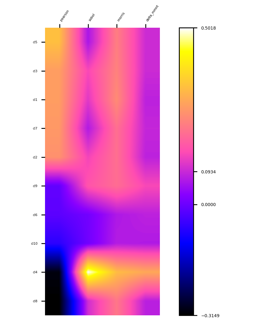
Step 2. Get to know the data by visualizing correlations and sensitivities:

from sklearn.gaussian_process.kernels import Matern, Sum, ExpSineSquared
from sklearn.kernel_ridge import KernelRidge
from sklearn.model_selection import RandomizedSearchCV
# use a regressor to approximate the data
param_grid_kr = {"alpha": np.logspace(-4, 1, 20),
              "kernel": [Sum(Matern(), ExpSineSquared(l, p))
                         for l in np.logspace(-2, 2, 10)
                         for p in np.logspace(0, 2, 10)]}
rgs = RandomizedSearchCV(KernelRidge(),
        param_distributions=param_grid_kr, n_iter=10, cv=2)
# ask for specific weights to be calculated and recorded
MLTr.FeatureWeights(regressor=rgs,
        weights=('pearson', 'sobol', 'morris', 'delta-mmnt'))
# visualise
plt1 = MLTr.heatmap(sort_by='pearson')
plt1.show()
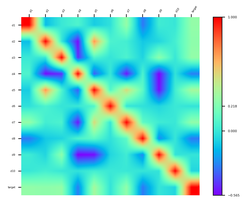
cor = df.corr()
plt2 = p = MLTr.heatmap(cor, idx_col=None, cmap='rainbow')
plt2.show()

Step 3. Examine and log a random forest model and its metrics:

from sklearn.ensemble import RandomForestClassifier
from sklearn.model_selection import cross_val_score, ShuffleSplit
# retrieve data
X, y = MLTr.get_data()
# init classifier
clf = RandomForestClassifier(n_estimators=50)
# log the classifier
clf = MLTr.LogModel(clf, "RandomForestClassifier(50)")
# find the average metrics
print(MLTr.LogMetrics(clf, cv=ShuffleSplit(5, .25)))
# {'accuracy': 0.8816, 'auc': 0.9504791437613562, 'precision': 0.9029848807772192,
# 'f1': 0.8782525829634803, 'recall': 0.8554950898148654, 'mcc': 0.7640884799286114,
# 'logloss': 4.089427586800243, 'variance': None, 'max_error': None, 'mse': None,
# 'mae': None, 'r2': None}

Step 4. Search for best (in terms of accuracy) classifier as a combination of naive_bayes.GaussianNB, linear_model.LogisticRegression, lightgbm.LGBMClassifier, preprocessing.StandardScaler, and preprocessing.Normalizer:

from SKSurrogate import *
# set up the confic dictionary
config = {
    # estimators
    'sklearn.naive_bayes.GaussianNB': {
        'var_smoothing': Real(1.e-9, 2.e-1)
    },
    'sklearn.linear_model.LogisticRegression': {
        'penalty': Categorical(["l1", "l2"]),
        'C': Real(1.e-6, 10.),
        "class_weight": HDReal((1.e-5, 1.e-5), (20., 20.))
    },
    "lightgbm.LGBMClassifier": {
        "boosting_type": Categorical(['gbdt', 'dart', 'goss', 'rf']),
        "num_leaves": Integer(2, 100),
        "learning_rate": Real(1.e-7, 1. - 1.e-6),  # prior='uniform'),
        "n_estimators": Integer(5, 250),
        "min_split_gain": Real(0., 1.),  # prior='uniform'),
        "subsample": Real(1.e-6, 1.),  # prior='uniform'),
        "importance_type": Categorical(['split', 'gain'])
    },
    # preprocessing
    'sklearn.preprocessing.StandardScaler': {
        'with_mean': Categorical([True, False]),
        'with_std': Categorical([True, False]),
    },
    'sklearn.preprocessing.Normalizer': {
        'norm': Categorical(['l1', 'l2', 'max'])
    },
}
# initiate and perform the search
A = AML(config=config, length=3, check_point='./sample/', verbose=1)
A.eoa_fit(X, y, max_generation=15, num_parents=20)
# retrieve and log the best
eoa_clf = A.best_estimator_
eoa_clf = MLTr.LogModel(eoa_clf, "Best of EOA Surrogate Search")
print(MLTr.LogMetrics(eoa_clf, cv=ShuffleSplit(5, .25)))
MLTr.PreserveModel(eoa_clf)
# {'accuracy': 0.8824, 'auc': 0.9207884992789751, 'precision': 0.8930688738450767,
# 'f1': 0.8789651291713657, 'recall': 0.8664344690110679, 'mcc': 0.7657250436230718,
# 'logloss': 4.061801043429923, 'variance': None, 'max_error': None, 'mse': None,
# 'mae': None, 'r2': None}

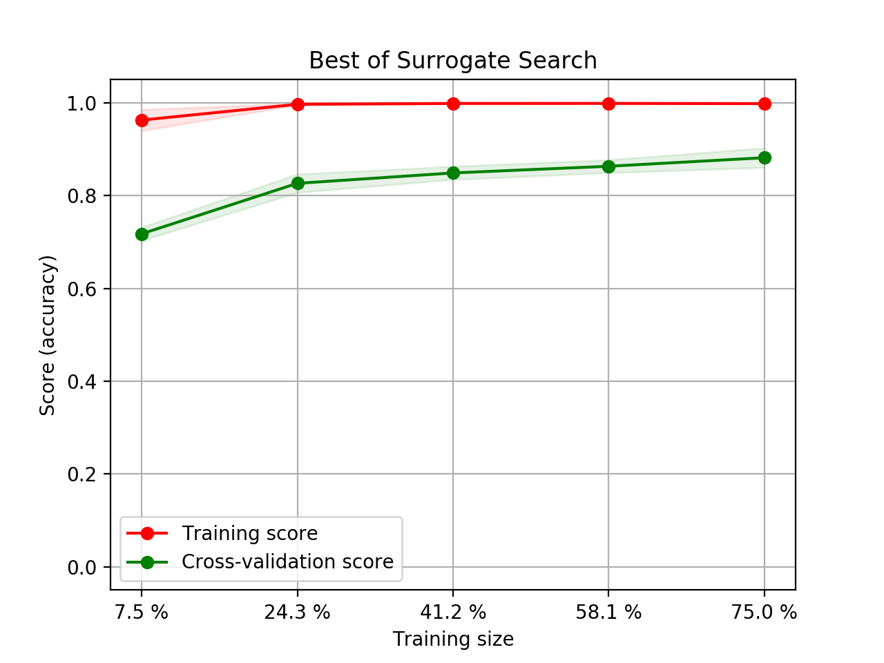
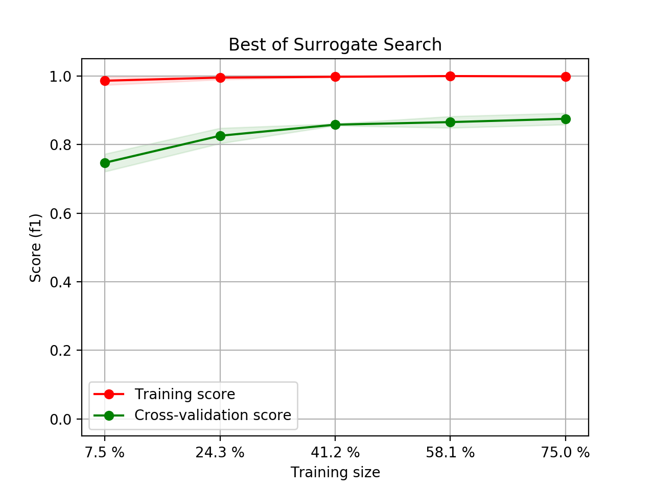
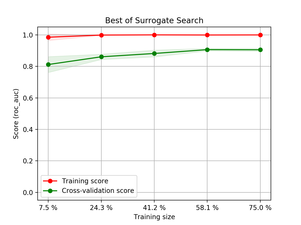
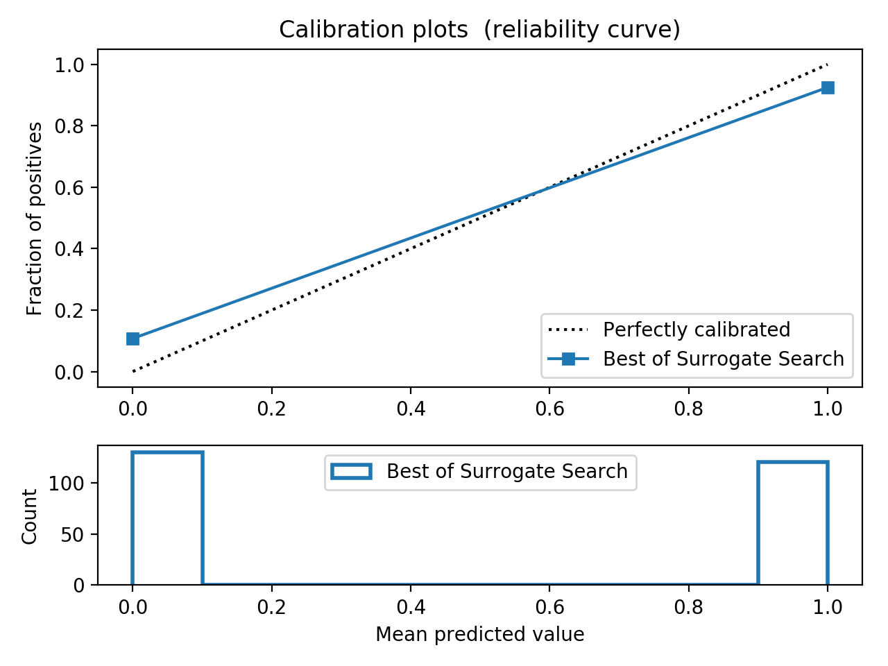
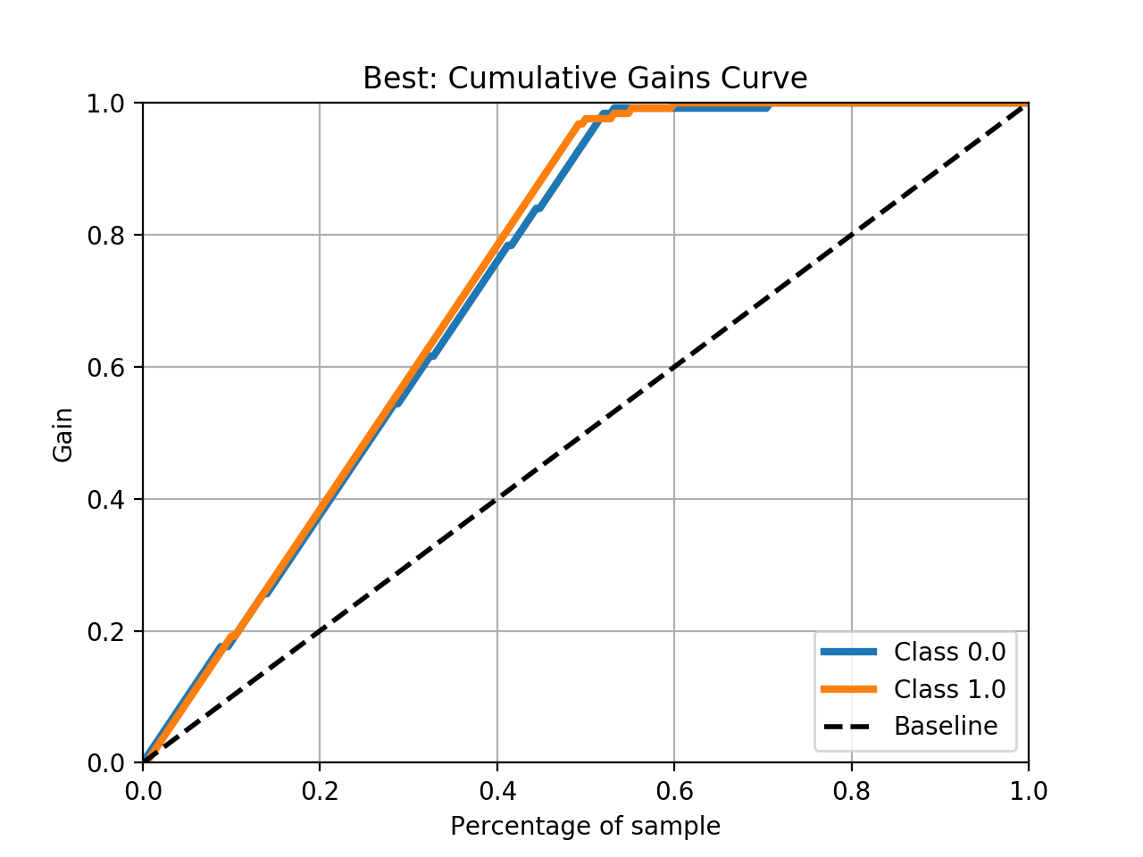
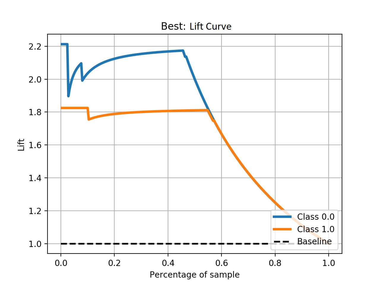
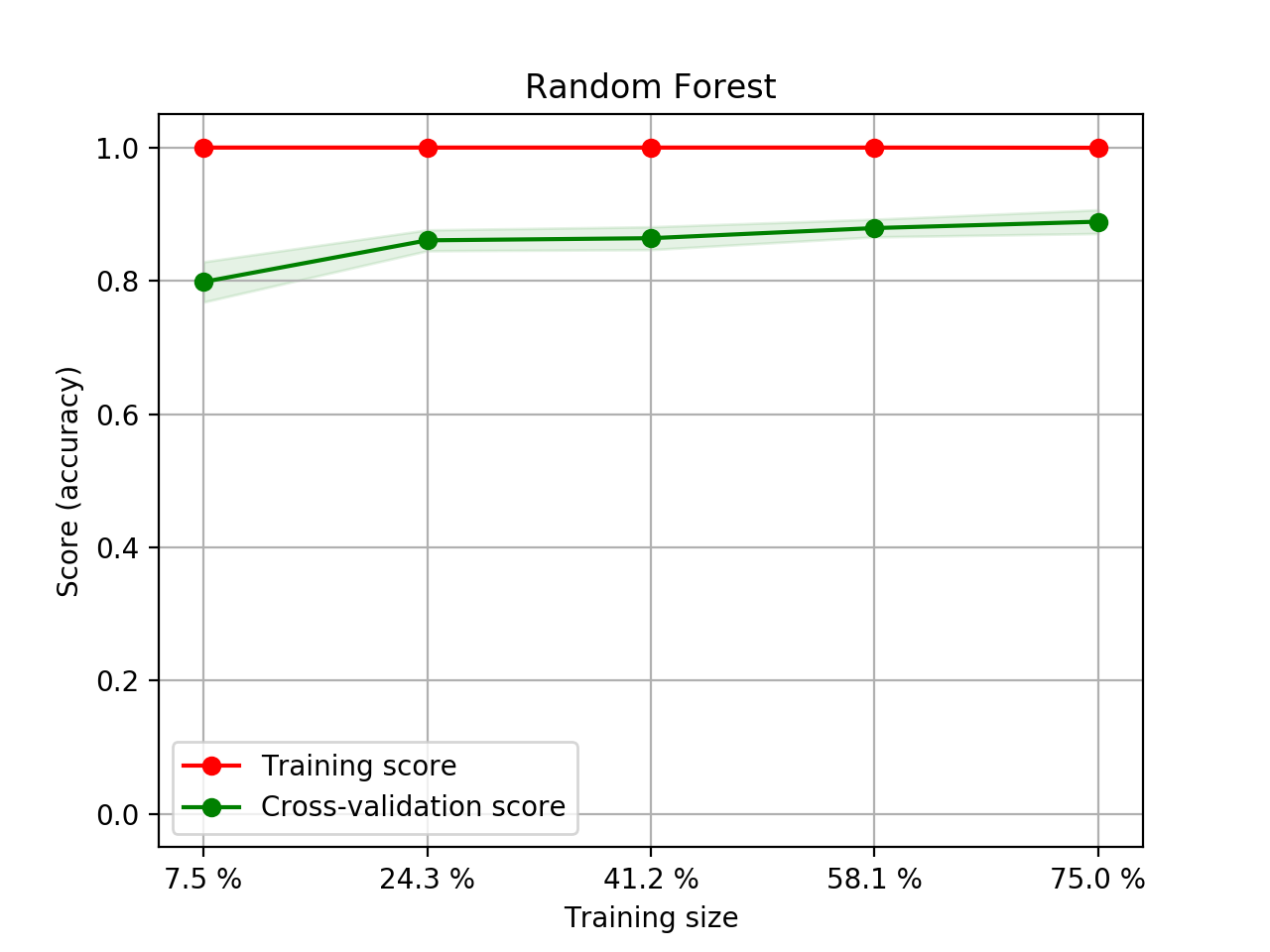
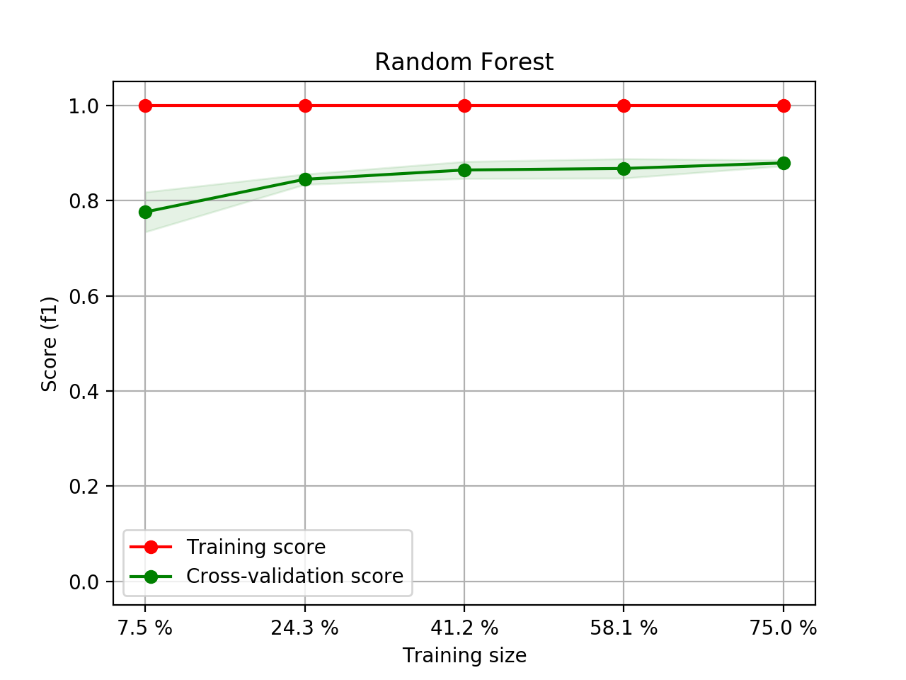
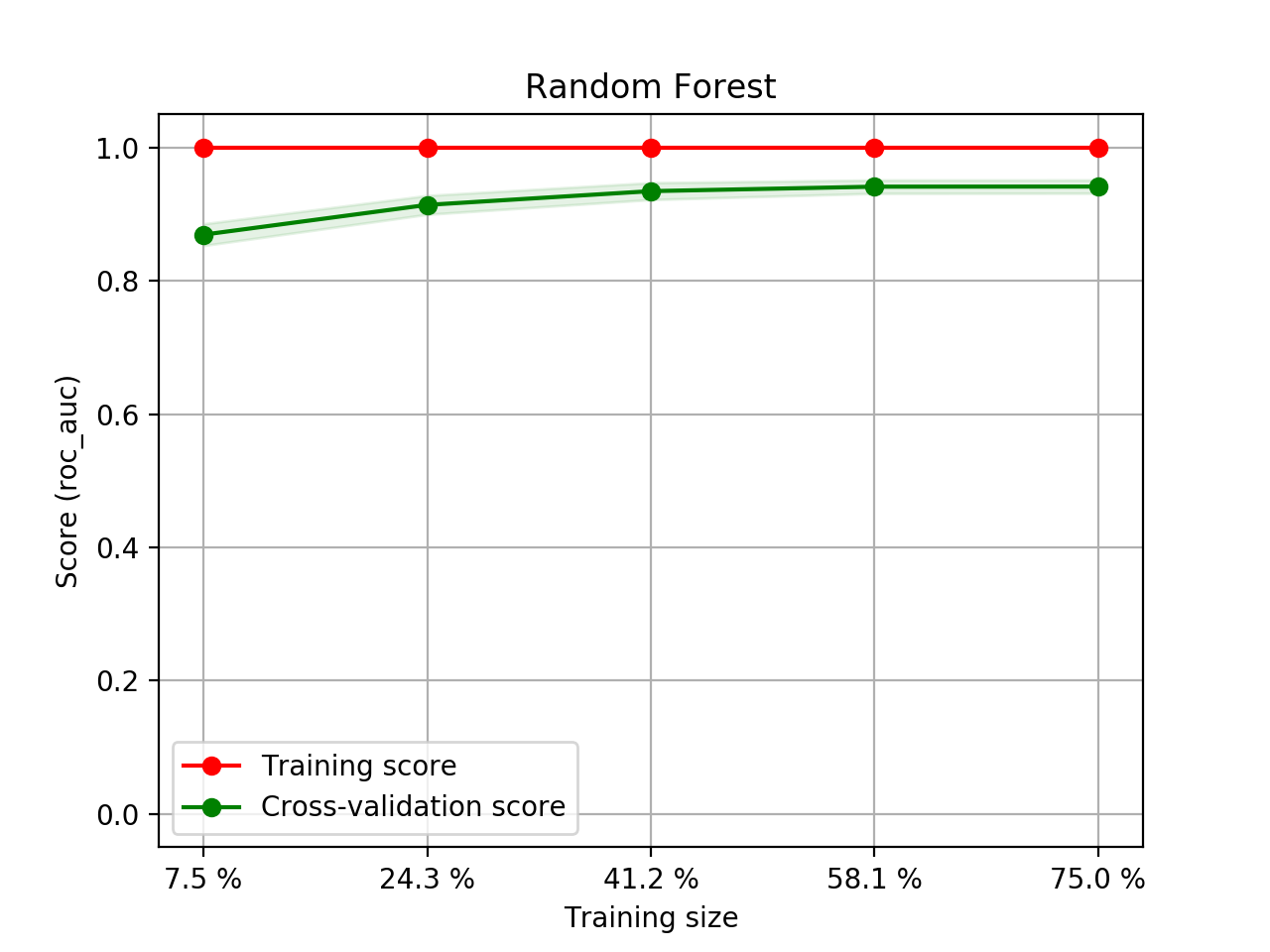
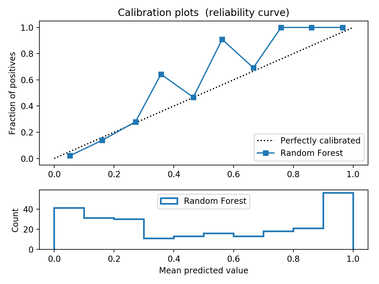
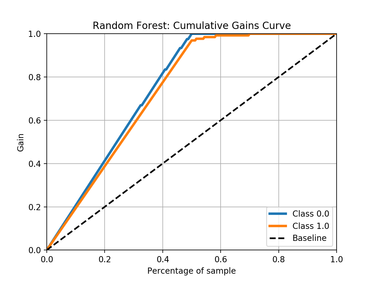
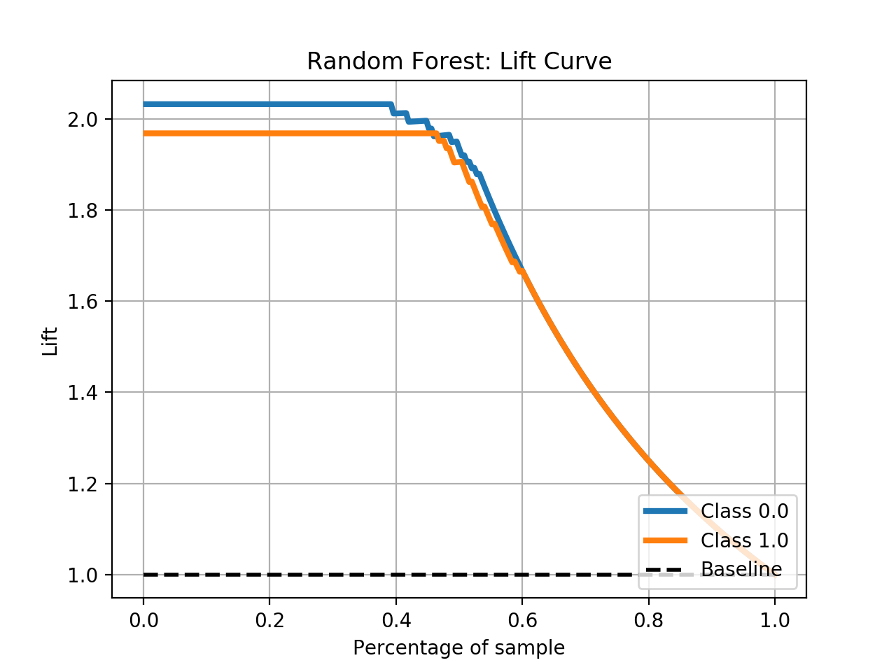
Step 5. Plot learning curves for accuracy, \(F_1\), area under ROC, calibration lift and

cumulative curves for the two models:

# the best of EOA Surrogate Search
MLTr.plot_learning_curve(eoa_clf, "Best of Surrogate Search", cv=ShuffleSplit(5, .25), measure='accuracy')
MLTr.plot_learning_curve(eoa_clf, "Best of Surrogate Search", cv=ShuffleSplit(5, .25), measure='f1')
MLTr.plot_learning_curve(eoa_clf, "Best of Surrogate Search", cv=ShuffleSplit(5, .25), measure='roc_auc')
MLTr.plot_calibration_curve(eoa_clf, "Best of Surrogate Search")
MLTr.plot_cumulative_gain(eoa_clf, title="Best: Cumulative Gains Curve")
MLTr.plot_lift_curve(eoa_clf, title="Best: Lift Curve")
# Random Forest
MLTr.plot_learning_curve(clf, "Random Forest", cv=ShuffleSplit(5, .25), measure='accuracy')
MLTr.plot_learning_curve(clf, "Random Forest", cv=ShuffleSplit(5, .25), measure='f1')
MLTr.plot_learning_curve(clf, "Random Forest", cv=ShuffleSplit(5, .25), measure='roc_auc')
MLTr.plot_calibration_curve(clf, "Random Forest")
MLTr.plot_cumulative_gain(clf, title="Random Forest: Cumulative Gains Curve")
MLTr.plot_lift_curve(clf, title="Random Forest: Lift Curve")

The Best of EOA

Random Forest

SVM Classifier with RBF v.s. SGDClassifier with Kernels

We try to see whether SVM classifiers with RBF kernel and SGDClassifres with kernel can compare. We set up a quick SKSurrogate search with SVC and NuSVC as classifiers and another quick SKSurrogate search over SGDClassifier, Nystroem and RBFSampler kernels:

import numpy as np
from SKSurrogate import *
import warnings
warnings.filterwarnings("ignore", category=Warning)

from sklearn.model_selection import RandomizedSearchCV
from sklearn.kernel_ridge import KernelRidge
from sklearn.gaussian_process.kernels import Matern, Sum, ExpSineSquared
param_grid_krr = {"alpha": np.logspace(-4, 0, 5),
                  "kernel": [Sum(Matern(), ExpSineSquared(l, p))
                             for l in np.logspace(-2, 2, 10)
                             for p in np.logspace(0, 2, 10)]}
regressor = RandomizedSearchCV(KernelRidge(), param_distributions=param_grid_krr, n_iter=7, cv=2)

config = {
    # estimators
    'sklearn.svm.SVC': {
        "C": Real(1e-6, 20.),
        "gamma": Real(1e-6, 10.),
        "tol": Real(1e-6, 10.),
        "class_weight": HDReal((1.e-5, 1.e-5), (20., 20.))
    },
    'sklearn.svm.NuSVC': {
        'nu': Real(1.e-5, 1.),
        "gamma": Real(1e-6, 10.),
        "tol": Real(1e-6, 10.),
        "class_weight": HDReal((1.e-5, 1.e-5), (20., 20.))
    },
    # preprocessing
    'sklearn.preprocessing.StandardScaler': {
        'with_mean': Categorical([True, False]),
        'with_std': Categorical([True, False]),
    },
    'sklearn.feature_selection.VarianceThreshold': {
        'threshold': Real(0., .3)
    },
    'sklearn.preprocessing.Normalizer': {
        'norm': Categorical(['l1', 'l2', 'max'])
    },
}

MLTr = mltrack('sample', db_name="sample.db")
X, y = MLTr.get_data()


A_svm = AML(config=config, length=3, check_point='./svm/', verbose=1)
A_svm.eoa_fit(X, y, max_generation=10, num_parents=10)
print(A_svm.get_top(4))

Which results in:

OrderedDict([(('sklearn.feature_selection.VarianceThreshold',
           'sklearn.preprocessing.Normalizer',
           'sklearn.svm.SVC'),
          (Pipeline(memory=None,
                steps=[('stp_0', VarianceThreshold(threshold=0.20066923736000097)), ('stp_1', Normalizer(copy=True, norm='l2')), ('stp_2', SVC(C=15.110221076172207, cache_size=200,
             class_weight={0.0: 13.581338880577112, 1.0: 3.1546898782179706},
             coef0=0.0, decision_function_shape='ovr', degree=3, gamma=10.0,
             kernel='rbf', max_iter=-1, probability=False, random_state=None,
             shrinking=True, tol=1e-06, verbose=False))]),
           -0.9253333333333333)),
         (('sklearn.preprocessing.StandardScaler',
           'sklearn.preprocessing.Normalizer',
           'sklearn.svm.SVC'),
          (Pipeline(memory=None,
                steps=[('stp_0', StandardScaler(copy=True, with_mean=True, with_std=False)), ('stp_1', Normalizer(copy=True, norm='l1')), ('stp_2', SVC(C=14.396152757785778, cache_size=200,
             class_weight={0.0: 11.644799650485178, 1.0: 14.834346896165036},
             coef0=0.0, decision_function_shape='ovr', degree=3,
             gamma=1.387860853481898, kernel='rbf', max_iter=-1, probability=False,
             random_state=None, shrinking=True, tol=1.3386685658572253, verbose=False))]),
           -0.9253333333333333)),
         (('sklearn.svm.NuSVC',
           'sklearn.preprocessing.Normalizer',
           'sklearn.svm.SVC'),
          (Pipeline(memory=None,
                steps=[('stp_0', StackingEstimator(decision=True,
                    estimator=NuSVC(cache_size=200,
              class_weight={0.0: 16.514247793012903, 1.0: 19.743755570932407},
              coef0=0.0, decision_function_shape='ovr', degree=3,
              gamma=2.879810799993445, kernel='rbf', max_iter=-1,
              nu=5.366323874825201e-05, pr...robability=False,
             random_state=None, shrinking=True, tol=0.0002612195258127529,
             verbose=False))]), -0.9226666666666666)),
         (('sklearn.feature_selection.VarianceThreshold',
           'sklearn.preprocessing.Normalizer',
           'sklearn.svm.NuSVC'),
          (Pipeline(memory=None,
                steps=[('stp_0', VarianceThreshold(threshold=0.10372588511430014)), ('stp_1', Normalizer(copy=True, norm='l2')), ('stp_2', NuSVC(cache_size=200,
              class_weight={0.0: 4.756565216129669, 1.0: 14.36176825433476},
              coef0=0.0, decision_function_shape='ovr', degree=3,
              gamma=5.437271690133034, kernel='rbf', max_iter=-1,
              nu=0.6557563687772239, probability=False, random_state=None,
              shrinking=True, tol=2.1918030657741365, verbose=False))]),
           -0.9186666666666666)))])

And for SGDClassifier:

import numpy as np
from SKSurrogate import *
import warnings
warnings.filterwarnings("ignore", category=Warning)

from sklearn.model_selection import RandomizedSearchCV
from sklearn.kernel_ridge import KernelRidge
from sklearn.gaussian_process.kernels import Matern, Sum, ExpSineSquared
param_grid_krr = {"alpha": np.logspace(-4, 0, 5),
                  "kernel": [Sum(Matern(), ExpSineSquared(l, p))
                             for l in np.logspace(-2, 2, 10)
                             for p in np.logspace(0, 2, 10)]}
regressor = RandomizedSearchCV(KernelRidge(), param_distributions=param_grid_krr, n_iter=7, cv=2)

config = {
    # estimators
    'sklearn.linear_model.SGDClassifier': {
        'loss': Categorical(['hinge', 'log', 'modified_huber', 'squared_hinge', 'perceptron']),
        'penalty': Categorical(['none', 'l2', 'l1', 'elasticnet']),
        'alpha': Real(1.e-5, .9999),
        'l1_ratio': Real(0., 1.),
        'tol': Real(1.e-5, 1.),
        'class_weight': HDReal((1.e-5, 1.e-5), (20., 20.))
    },
    # preprocessing
    'sklearn.preprocessing.StandardScaler': {
        'with_mean': Categorical([True, False]),
        'with_std': Categorical([True, False]),
    },
    'sklearn.feature_selection.VarianceThreshold': {
        'threshold': Real(0., .3)
    },
    'sklearn.preprocessing.Normalizer': {
        'norm': Categorical(['l1', 'l2', 'max'])
    },
    # Transformers
    'sklearn.kernel_approximation.Nystroem': {
        'kernel': Categorical(['rbf', 'poly', 'sigmoid']),
        'gamma': Real(1.e-6, 10.),
        'n_components': Integer(10, 120)
    },
    'sklearn.kernel_approximation.RBFSampler': {
        'gamma': Real(1.e-6, 10.),
        'n_components': Integer(10, 120)
    },
}

MLTr = mltrack('sample', db_name="sample.db")
X, y = MLTr.get_data()


A_sgd = AML(config=config, length=3, check_point='./svm/', verbose=2)#, cat_cols=[5])
A_sgd.fit(X, y)
print(A_sgd.get_top(4))

Which results in:

OrderedDict([(('sklearn.linear_model.SGDClassifier',
               'sklearn.kernel_approximation.Nystroem',
               'sklearn.linear_model.SGDClassifier'),
              (Pipeline(memory=None,
                    steps=[('stp_0', StackingEstimator(decision=True,
                        estimator=SGDClassifier(alpha=1.0186882143892309e-05, average=False,
                      class_weight={0.0: 1e-05, 1.0: 1e-05}, early_stopping=False,
                      epsilon=0.1, eta0=0.0, fit_intercept=True,
                      l1_ratio=0.16668760571866542, learning_rate='op...om_state=None, shuffle=True,
                      tol=1.0, validation_fraction=0.1, verbose=0, warm_start=False))]),
               -0.8946666666666667)),
             (('sklearn.preprocessing.Normalizer',
               'sklearn.kernel_approximation.RBFSampler',
               'sklearn.linear_model.SGDClassifier'),
              (Pipeline(memory=None,
                    steps=[('stp_0', Normalizer(copy=True, norm='l1')), ('stp_1', RBFSampler(gamma=5.09346829872262, n_components=120, random_state=None)), ('stp_2', SGDClassifier(alpha=1e-05, average=False,
                      class_weight={0.0: 6.299501235657723, 1.0: 14.399482243823948},
                      early_stopping=False, epsilon=0.1,..._state=None, shuffle=True,
                      tol=1e-05, validation_fraction=0.1, verbose=0, warm_start=False))]),
               -0.8946666666666667)),
             (('sklearn.kernel_approximation.Nystroem',
               'sklearn.preprocessing.Normalizer',
               'sklearn.linear_model.SGDClassifier'),
              (Pipeline(memory=None,
                    steps=[('stp_0', Nystroem(coef0=None, degree=None, gamma=7.102137254366565, kernel='poly',
                    kernel_params=None, n_components=51, random_state=None)), ('stp_1', Normalizer(copy=True, norm='l2')), ('stp_2', SGDClassifier(alpha=0.4030001737762923, average=False,
                      class_weight={0.0: 16.5900487...shuffle=True, tol=0.6700383879862661,
                      validation_fraction=0.1, verbose=0, warm_start=False))]),
               -0.8906666666666667)),
             (('sklearn.preprocessing.Normalizer',
               'sklearn.kernel_approximation.Nystroem',
               'sklearn.linear_model.SGDClassifier'),
              (Pipeline(memory=None,
                    steps=[('stp_0', Normalizer(copy=True, norm='l2')), ('stp_1', Nystroem(coef0=None, degree=None, gamma=5.928661960771689, kernel='poly',
                    kernel_params=None, n_components=117, random_state=None)), ('stp_2', SGDClassifier(alpha=0.5112964074641659, average=False,
                      class_weight={0.0: 3.2816638...shuffle=True, tol=0.7276228102426916,
                      validation_fraction=0.1, verbose=0, warm_start=False))]),
               -0.884))])

This shows a \(3.06\%\) loss in accuracy